Model Reference Adaptive Control.
Model Reference Adaptive Control (MRAC) is one of the primary approaches to Adaptive Control. The basic idea of MRAC is to design a controller to make an uncertain nonlinear plant to follow a Reference model characterized by designed natural frequency and damping. We can define the nonlinear plant model (to be controlled!) as
\[\begin{align*} \dot{x}(t) = f(x)+Bu(t) \end{align*}\]Where \(x(t) \in \mathcal{D}_x \in \mathbb{R}^n\), \(u(t) \in \mathbb{R}^m\) and \(f: \mathbb{R}^n \rightarrow \mathbb{R}^n\) is Lipschitz.
The unknown nonlinear plant model can be re-written in form of nominal dynamics and model uncertainties as,
\[\begin{align*} \dot{x}(t) = Ax(t)+B(u(t) + \Delta(x) \end{align*}\]Where \(\begin{align*}\Delta(x) \triangleq f(x(t))-Ax(t)\end{align*}\) is the model uncertainty.
The MRAC controller aims to enforce the unknown nonlinear dynamic system to track a designed reference model given as
\[\begin{align*} \dot{x}_{rm}(t) = A_{rm}x_{rm}(t)+B_{rm}r(t) \end{align*}\]The total control is designed to be of the form \(u(t) = -kx(t)+k_gr(t)-\nu_{ad}\),
Where \(k, k_g\) are designed to satisfy the following matching condition
\[A_{rm} = A-Bk, B_{rm}=Bk_g\]The MRAC focuses on designing the adaptive part of the controller \(\nu_{ad}\), which aims at canceling the model uncertainties.
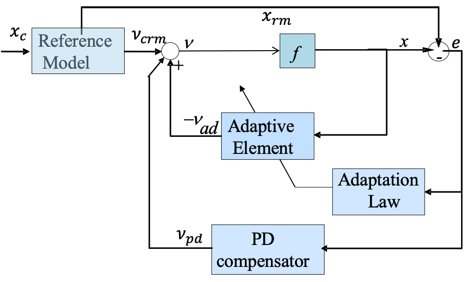
Traditionally classical MRAC handles the uncertainty as modeled as a single layer neural network. The uncertainties can be modeled as structured and unstructured uncertainties as follows,
Structured Uncertainty
\[\begin{align*} \Delta(x(t)) = W^{*T}\sigma(x) \end{align*}\]Where \(W^{*} \in \mathbb{R}^{k \times m}\) are the unknown ideal weights, and \(\sigma(x):\mathbb{R}^k \rightarrow \mathbb{R}^m\) are known feature vector (specific to the plant dynamics)
Un-Structured Uncertainty
\[\begin{align*} \Delta(x(t)) = W^{*T}\phi(x) + \epsilon(x) \end{align*}\]Where \(W^{*} \in \mathbb{R}^{k \times m}\) are the unknown ideal weights, \(\phi(x):\mathbb{R}^k \rightarrow \mathbb{R}^m\) are designed feature vector (RBF are most popular choice) and \(\epsilon(x) \in \mathbb{R}^m\) is network approximation error(Universal Approximation Theorem)
Since we do not know the true ideal weights \(W^*\), we learn the approximation of true weights \(W\) online interacting with the system. The Weights are update in the direction of minimizing the instantaneous tracking \(e(t) = x(t)-x_{rm}(t)\).
The classical MRAC weight update law is given as,
\[\begin{align*} \dot{W} = -\Gamma\phi(x)e(t)^TPB \end{align*}\]where \(P\) is solution of Lyapunov equation \(A_{rm}^TP+PA_{rm}+Q = 0\), where \(Q, P > 0\).
The tricky part of MRAC is when the uncertainty is treated as unstructured uncertainty, which requires the designer to select the basis vectors and tune hyperparameter judiciously. We provide results for MRAC controller performance on a toy example of the “Wing-Rock” dynamics of delta-wing aircraft.
We will assume three cases
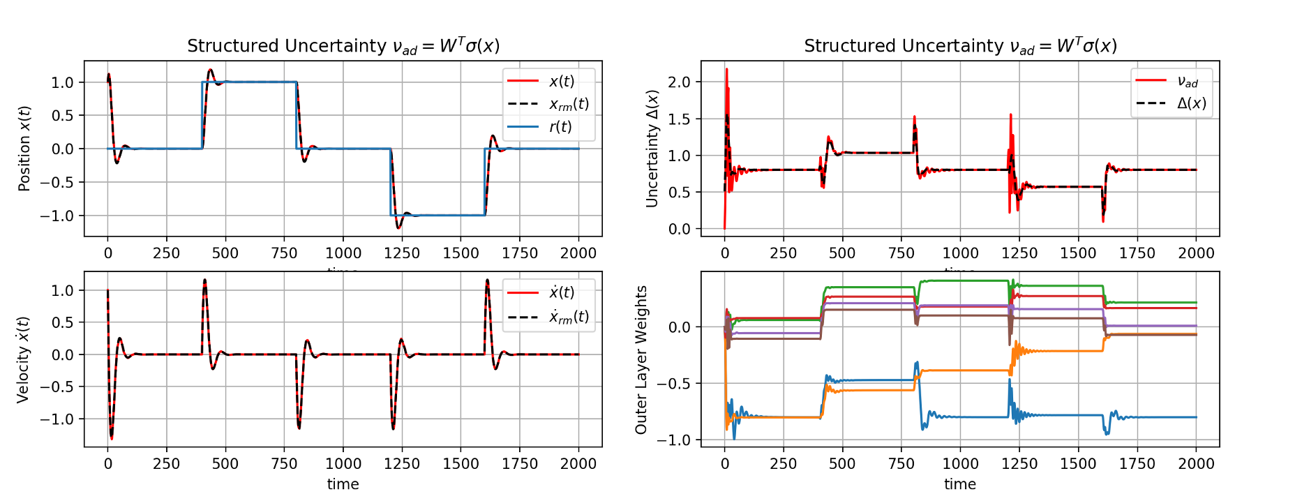
- Structured uncerainty (when the structure of uncertainty is known) \(\nu_{ad} = W^T\sigma(x)\)
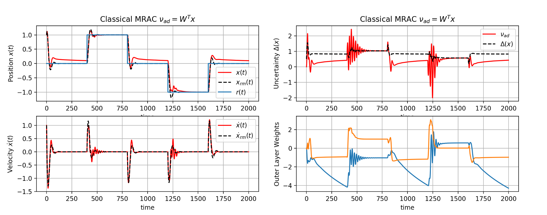
- Classical MRAC with linear in state network \(\nu_{ad} = W^Tx\)
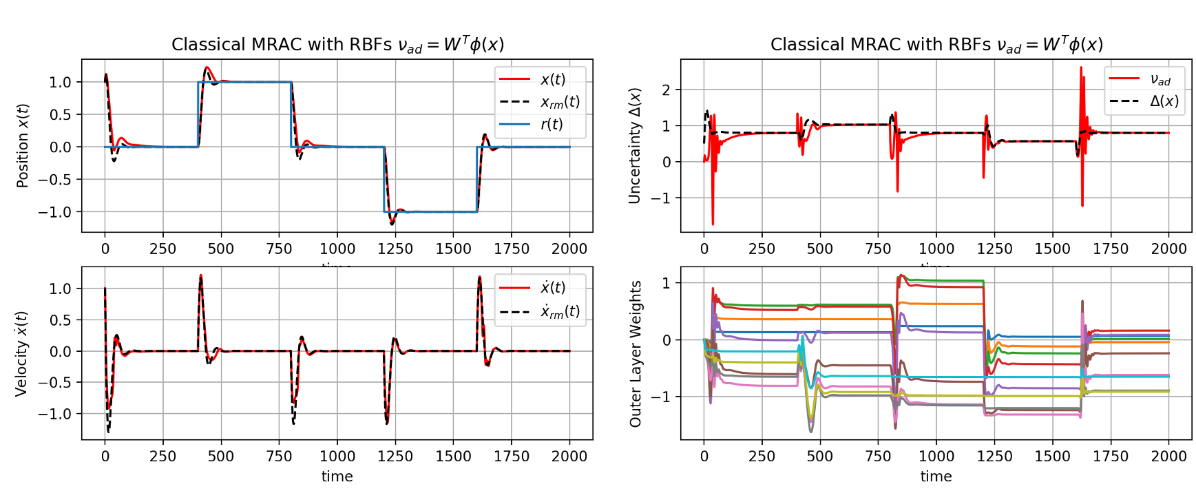
- Unstructured uncerainty (with RBF features) \(\nu_{ad} = W^T\phi(x)\)
The wing rock dynamics is defined as,
\[\begin{align*} \dot{\theta} &= p \\ \dot{p} &= L_{\delta_a}\delta_{a} + \Delta(x) \end{align*}\]where \(\Delta(x) = W^{*}_{0} + W^{*}_{1}\theta + W^{*}_{2}p + W^{*}_{3}\|\theta\|p + W^{*}_{4}\|p\|p + W^{*}_{5}\theta^3\)
For the Structured Uncertainty case, we use the known basis vector from the dynamics and estimate \(W_i\)’s online. Lets set \(\sigma(x) = [1, \theta, p, \|\theta\|p, \|p\|p, \theta^3]\) and learning rate \(\Gamma = 100\), the MRAC controller results in state tracking and disturbance, weight approximation presented in the plots as follows,
For unstructured case, the most popular choice of feature for the classical MRAC controller (like L1-Adaptive Controller) is the system state itself. As we can see in the plots below for the given nonlinear disturbance, a linear in-state representation of uncertainty is clearly not sufficient.
In the more general case where the uncertainty \(\Delta(x)\) is assumed to be continuously differentiable and defined over a compact domain, the adaptive part of the control law can be formed using Radial basis functions (RBF) or shallow networks ( SHL). The following plots are for RBF-NN MRAC controller. Given a dynamical system, and with a careful choice of feature hyperparameters, we can construct an NN based adaptive controller that performs well with minimal tracking error.
We leave the stability aspects of the controller out of this article. Interested readers can refer [Concurrent Learning without Persistency of Excitation] for further details.
Further reading Deep Model Reference Adaptive Control